GIS II: Network Analysis Part II

Introduction

This week's exercise is building off the previous exercises and involves more network analysis. Since transportation from sand mines to rail terminals have a significant adverse impact on local roads, the goal of this exercise is to find the closest route from mine to terminal and then attach a transportation cost for each county. Data sets involved in this exercise are: Sand Mine locations, Railroad Terminals, County shapefiles, and Street Network dataset.The data sources for the Street dataset and County shapefiles are from ESRI.

Methodology

Last week, we ran the Closest Facility function found in the Network Analysis window to get an output of roads representing the shortest distance from mines to terminals. However, the result was not transformed immediately into a shapefile or feature class. To do this, we utilized Model Builder to run the process and then subsequently export the results to a feature class within our geodatabase. In Model Builder, the first thing I did was add the Closest Facility tool from ArcToolbox. The streets dataset was added as the input and the only parameter changed was setting 'travel to facility'. The mine locations were added next using the Add Locations tool. The input was filled with the mines feature class and the sub layer set to incidents. After this information was filled in, it was connected to the Closest Facility layer mentioned above. The next step was to use Add Locations again, this time for the rail terminals. The terminal feature was added to the input and the sub layer set to facilities. This was then connected to the previous Add Locations output. This will become much clearer in Fig. 1 displaying the workflow of the model. Once all the inputs were defined, the Solve tool could then be run to produce an output showing the shortest distance routes from each mine to the closest terminal.

Fig. 1- Model depicting process of creating a Closest Facility layer.

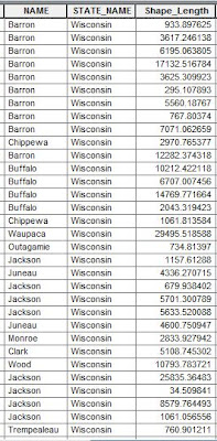
The intermediate output, Closest Facility 2 (3), after the Solve function, contains the roads showing shortest distance. To export this data as a feature class, the Select Data tool was added to the model to select the routes and then copy them into the geodatabase. The resulting feature class is denoted at the end of the workflow, closest_faciltity_routes. Once the desired output was generated, the next task was to figure out the length of roads being traveled for each county in order to assign a cost to each county. Once again, Model Builder was used for this process as well. What was then decided to be the best tool for this particular process was the Intersect tool which basically slices the routes into sections contained within each county. The Intersect tool was added to the model and then the closest routes and county feature classes were added to the inputs. This resulted in a feature class containing a table of all pieces of a route lying inside each county.

Fig. 2 - Building a model to run the Intersect and Summarize Statistics tools.

Results/Discussion

The results of the first model can be seen in Fig. 3 below.


Fig. 3 - Results from the first model.

 

 

The results from the second model produced a feature class containing a table that showed each parcel of road within each county and the associated length in meters.


Fig. 4 - Table from the intersected features showing length (m) of each road section by county.

This was the correct output we were looking for but needed to condense the table so that only one entry for each county would show up with a total road length quantity for each county. This was done by adding the Summarize Statistics tool to the model. This tool added up all of the pieces of road by county and then the values were converted to miles by adding another field to the table and entering in the conversion formula.


Fig. 5 - Table after running Summarize Statistics tool.

This table is a lot more cleaned up and orderly and will be way easier to assign costs to each county now that there is only one record for each county.

The costs assigned for each county are derived from a hypothetical set of parameters. We are assuming taht each sand mine takes 50 truck trips per year, to the terminal and back. Each mile the truck travels has a cost of 2.2 cents attached to it. This is a pretty simple expression to figure out the cost for each county: ([Miles]*2)(2.2/100)*50.

Fig. 6 - Table with a new Cost field ($) added, calculated by the formula above.

Given that this is a hypothetical situation, the cost figures do not really represent the actual costs that each county can expect for road repair each year. However, being able to do a network analysis like this and assign costs is a very powerful tool to help make aware the potential damage that transportation of sand is having on local roads. Obviously, some counties will experience a lot more stress on their roads then do other counties due to the location of the closest terminals. This information could inform the DOT to limit use or truck weight on certain roads to help minimize the high costs.

Conclusion

This exercise was really cool and powerful to work through. Getting a better understanding of Network Analysis and its capabilities can be monumentally beneficial if ever confronted with a project like this. Working with Model Builder was a bit difficult at first but ended up really streamlining and expediting the processes involved. Otherwise, each tool would have had to be run separately and then the geodatabase would have been inundated with uneccesary intermediate feature classes. Also, it was very beneficial in having to develop a formula and then apply it to a new field within a dBase table. It's always a good feeling to see the finished product after having started from scratch.