GIS II: Suitability Analysis with Rasters Part II

Introduction

This post is the second part of an exercise involving finding suitable land for a new sand mine and also for developing a hazard index for a new sand mine location. The Suitability Index was created in the previous post and now the focus is on the impact of sand mining by creating a Hazard Index based on a set of community and environmental factors: Proximity to Streams, Prime Farmland, Proximity to Residential Areas, Proximity to Schools, Visibility from Trails and Parks, and Wetlands. For each criteria, an impact figure will be assessed (3=High, 2=Medium, 1=Low) to determine the impact a sand mine would have if located in a certain area. High impact locations will be locations where mines should not be located. The rankings will then be summed up in order to create a Hazard Index. The study area is Trempeleau County, WI shown below.

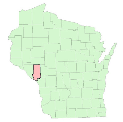Fig. 1 - Trempeleau County, the study area, shown in red.

Methodology

Once ArcMap was opened, the environments were set so that the workspace was assigned to my personal geodatabase, the coordinate system set to UTM 15N, output cell size at 30m, and the raster analysis mask set to the Trempeleau County feature class. Once the preliminary settings were defined, the next step was to tackle each objective one by one. All distances are in meters (m).
The first objective was to measure the impact on streams. The geodatabase for Trempeleau County was utilized to find the stream feature class called DNR-Hyro-junction. This feature contains many different types of streams such as combinations of Primary and Secondary streams, Perennial and Annual, and Overland and Instream flow. Using all of the combinations of streams meant that pretty much the whole county was streams. Running a Euclidean Distance on this would have not made much sense as the whole county would be considered a hazard area. Plus, not all of these streams are not around all of the time. To select the appropriate streams, a query was run to extract streams that were Perennial, Primary or Secondary, and Instream flow which would be the main streams in the county.

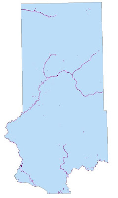Fig. 2 - Queried streams used for Objective 1. 

After the correct streams were selected, a Euclidean Distance was run based off of the streams feature class. Any time Euclidean Distance is used in this project, the processing extent needs to be greater than the size of Trempeleau County or else the extent will not extend to cover the whole county. From this, the Extract by Mask tool can be used to clip the Euclidean Distance to the extent of the county.

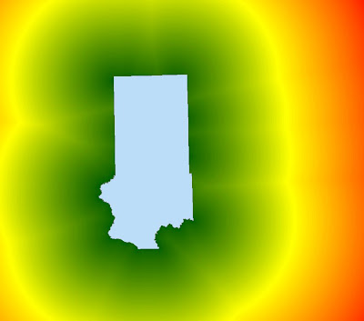Fig. 3 - The first Euclidean Distance to ensure complete coverage of Trempeleau County.

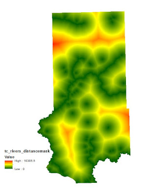Fig. 4 - Euclidean Distance from streams after Extract by Mask tool was used. 

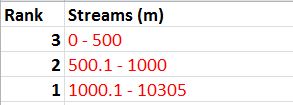
The next step was to reclassify the distances into 3 classes (High, Medium, Low). Since streams are such a precious resource, it was decided to give them a lot of breathing room. The following are the class breaks: (0-500) a 3, (500.1-1000) a 2, and (1000.1-10305) a 1.

Fig. 5 - Stream distance class breaks.

Fig. 6 - The model used to run Euclidean Distance and then reclassify the distances from streams.

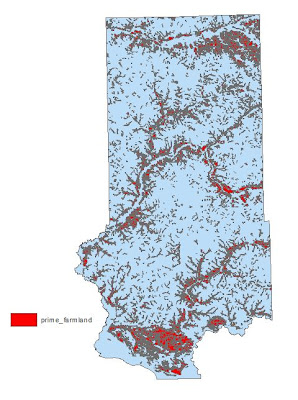
Objective 2 wants us to assess the risk to prime farmland. Once again, the Trempeleau County geodatabase was used to extract this information. There are varying types of farmland denoted by their production rates.Areas of prime farmland were identified through the attribute table and then extracted.

Fig. 7 - Prime farmland in Trempeleau County.

 Prime farmland can be disrupted by disturbing the soils. Once again, Euclidean Distance was used to determine the proper buffers. The classes were defined as: (0-100) a 3, (100.1-300) a 2, and (300-3515) a 1. It was felt that a 100m buffer was ample to protect areas of prime farmland. The Natural Breaks method was not used in this but rather rational thinking was applied to preserve these areas while at the same time not limiting potential locations. 

Fig. 8 - Class breaks for distance from prime farmland.

 

Fig. 9 - Model used to determine hazard to prime farmland.

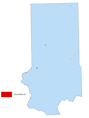
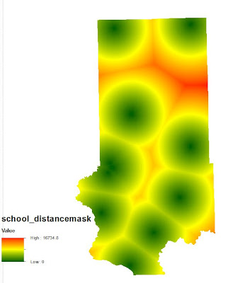
For Objective 3, the goal was to figure out the impact on schools. There is no schools feature class in the geodatabase so a different method needed to be used to determine school locations. A feature class called Parcels was located in the Trempeleau County geodatabase and was used to query out parcels which were owned by schools. School Districts could not be used as they contain the entire area closest to a particular school. Euclidean Distance was then run to be able to reclassify and rank distances.

Fig. 10 - Areas in red denote parcels owned by schools.

Fig. 11 - Distance from schools determined by the Euclidean Distance tool.

Since a mine must be located 640m away from a residential area for noise and dust concerns, the same distance will be applied to schools. Therefore the 3 classes were defined as: (0-640) = 0, (640.1-1000) = 3, (1000.1-1500) = 2, and (1500.1-16734 = 1. Once again subjective, yet logical thinking went into this.

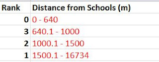Fig. 12 - Table ranking distance from schools.

Fig. 13 - Model used to develop a hazard index for schools. 

The goal for Objective 4 was to calculate distance from residential or populated areas. These areas are susceptible to noise and dust caused by mining operations. The distance a mine must be away from a residential area is at least 640 meters. There are several classes which contain information regarding residential areas. The LULC dataset includes such areas but also includes road networks with areas of residential so this is no good. The zoning feature class was not used either because the zoning polygons were too large and contained areas where there was no residence. Census data was also available but that too would have included too much area or too little depending on population density used to determine these areas. There was a feature called Plat in the geodatabase which was overlaid on top of the LULC raster. This feature did a very good job of outlining areas of residential without too much overestimating or underestimating. It was decided that this feature contained the least amount of erroneous areas and was used to represent residential areas.

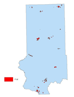Fig. - 14 - Plat parcels used to delineate areas of residential.

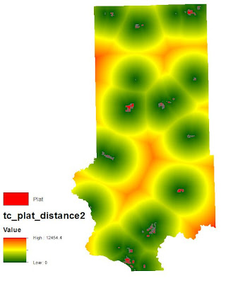Fig. 15 - Noise/Dust shed determined by Euclidean Distance.

The distances were reclassified into 4 classes: (0-640) = 0, (640.1-1000) = 3, (1000.1-1500) = 2, and (1500.1 - 12454) = 1. It was determined that only a short extension beyond the 640m should be deemed a high hazard since 640m is already a large buffer.

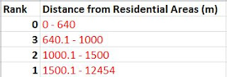Fig. 16 - Class breaks for distance from residential areas.

Fig. 17 - Model used to determine a noise/dust shed around residential areas. 

Objective 5 seeks to mitigate visibility of a sand mine from prime recreational areas such as trails and parks. In order to achieve this, a viewshed must be calculated from these feature classes. A viewshed uses elevation values from the DEM to determine areas that are visible and not visible from the feature classes. Running the Viewshed tool took an extremely long time on the Trails feature class. Since this tool only works on line or point features, the Parks feature class (polygon) needed to be converted into a point feature. The tool used for this conversion is called the Feature to Point tool located in Data Management. This tool assigned a point to the center of each park polygon.

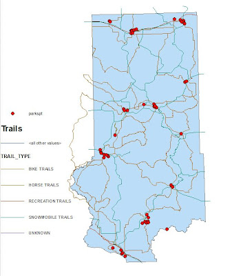Fig. 18 - Trails and Parks in Trempeleau County, WI.

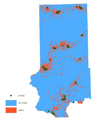Fig. 19 - Areas of visibility and invisibility from park locations.

The park viewshed was then reclassified as follows: (0) = 1, (1-6) = 2, and (6-12) = 3. The values above zero indicate the number of times that spot can be seen from any other point on the map. Therefore, the higher values are areas of high visibility and are thus assigned a high hazard value. 

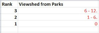Fig. 20 - Viewshed from Parks class breaks.

 

Fig. 21 - Model used to determine viewshed from parks.

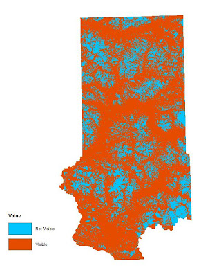Fig. 22 - Areas of visibility and invisibility from trails in Trempeleau County.

The viewshed for trails was reclassified as follows: (0) = 1, (1-35) = 2, and (35-1822) = 3.

Fig. 23 - Trail viewshed class breaks.

Fig. 24 - Model used to determine viewshed from trails.

For the final objective, we were given the freedom to choose one more variable to include in the analysis. I chose to assess the hazard to wetlands. Even though wetlands were addressed in the Suitability Index, the feature class in the Trempeleau County geodatabase is far more detailed than the wetlands delineated in the LULC map. Wetlands are very fragile and are a very important component to the ecosystem. For these reasons, I chose to assess the hazards to wetlands as they are a very valuable resource and must be protected. Euclidean Distance was run and then reclassified.

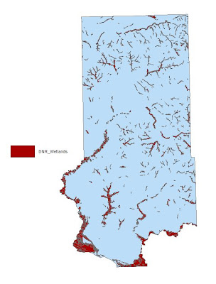Fig. 25 - Areas of wetlands in Trempeleau County.

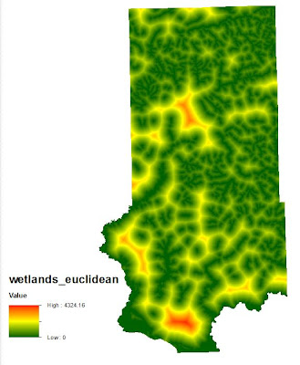Fig. 26 - Distance from wetlands.

The classification scheme for ranking hazards to wetlands is as follows: (0-300) = 3, (300.1-700) = 2, and (700.1 - 4324) = 1. It was decided that there should be a large buffer zone around wetlands to that any harmful constituents from a sand mine would be prevented from leaching into the wetlands.

Fig. 27 - Wetlands table class break rank.

Fig. 28 - Model used to determine hazards to wetlands.

After all of the criteria had been properly ranked, they were added together using the Raster Calculator tool. This tool sums up all of the values at each cell location and then outputs the sums in a new raster. The range of sums in this exercise can be from 7 to 21.

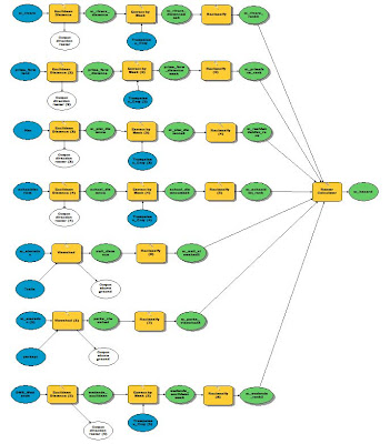Fig. 29 - Raster Calculator was used to add up all of the criteria rasters into a Hazard Index.

Results/Discussion

Below are the classified results from each objective and then the final Hazard Index. 



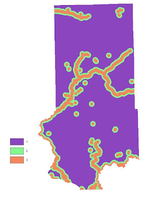Fig. 30 - Hazard Index for streams.

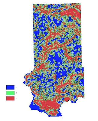Fig. 31 - Hazard Index for prime farmland.

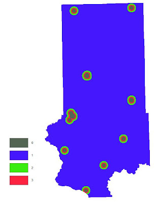Fig. 32 - Hazard Index for schools.

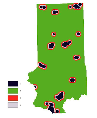Fig. 33 - Hazard Index for residential areas.

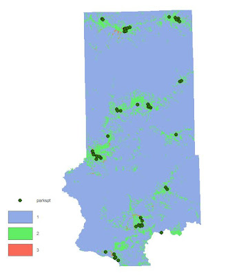Fig. 34 - Hazard Index for parks.

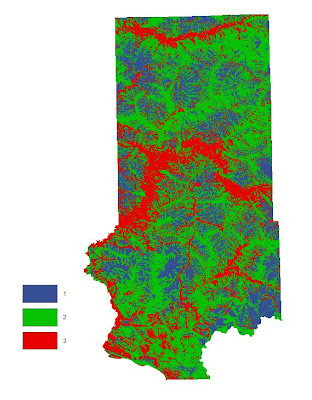Fig. 35 - Hazard Index for trails.

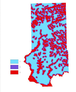Fig. 36 - Hazard Index for wetlands.  

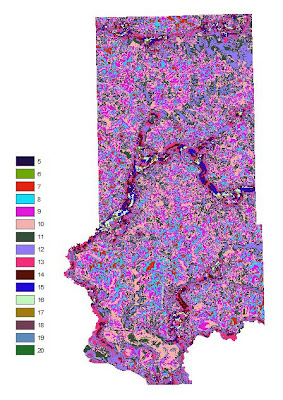Fig. 37 - Summed up values of all criteria.

Areas of residential and schools are off limits for building a mine so they need to be excluded from the final Hazard Index.

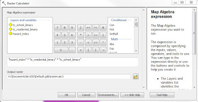Fig. 38 - Raster Calculator tool used to exclude schools and residential areas.

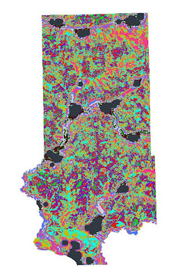Fig. 39 - Schools and residential areas excluded from  Hazard Index.

The map in Fig. 32 needs to be simplified and so it was reclassified as follows: (7-10) = 1, (11-14) = 2, and (15-20) = 3. I chose these values because the lowest possible value is 5 which is low hazard where if all 7 inputs contained a value of 1 it would equal 7. The highest value for Medium is 14 where if the value of a cell is 2 (Medium rank) in the same cell for each raster, then the value would equal 14. Any value above 14 is considered a High Hazard area.

Fig. 40 - Model used to reclassify summed up values into a 3 rank Hazard Index.

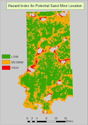Fig. 41 - Final Hazard Index map.

 

Here again, the class breaks chosen were subjective yet a logical though process was used to determine them. However, someone else could argue the breaks differently and thus create a different output. I thought there would be more high hazard areas in the final output. I was surprised that there was no location where the same cell for all inputs equaled 3 which would have given a summed value of 21. It appears that there are plenty of options for a new sand mine where the hazard would be minimal. This could look differently had the buffers around certain criteria been larger. I did not find it practical to extend a high hazard buffer a great distance from some of the features.

Conclusion

This exercise was a lot of fun to work through as we were given a lot of freedom in determining class breaks for the hazard rankings. This allowed us to really think about distances and try to visualize that which is kind of tough actually. However, this is a real world situation and it was very good experience processing a wide variety of data and deciding which data should be used to get the most accurate results.