GIS II: Suitability Analysis with Rasters

Introduction

Now that we have established where the mines are and also the closest railroad terminal to each mine location, it is time to find suitable land for future sand mines. There can be be countless paramater combinations used to determine where the most suitable locations are to accomodate a sand mine. Deciding on these factors can be a very subjective process. However, for the purpose of this project, we want to focus on some of the biggest factors, mostly environmental, that will determine which areas are best suited for a sand mine based on a ranking scale. We all know that a sand mine has major implications on the environment as well as it does to urban living as no one wants to live next to a noisy sand mining operation. The criteria that we will look at for a suitability model are: elevationk, land use/land cover, distance to rail terminals, slope, and depth to water table. Since we are limited by time constraints, the focus of this portion of the project will focus solely on Trempeleau County, WI.


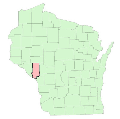Fig. 1 - Trempeleau County, the study area, shown in red.

All of the datasets have been downloaded from a variety of sources and are in raster format. The criteria was broken into class breaks and then ranked for suitability (High = 3, Medium = 2, Low = 1). The final step will be to combine the five raster datasets into a suitability index model. All of the processes will be run through Model Builder.

Methodology

The first thing that we did was to set the geoprocessing environments so that all of the processes could be streamlined more efficiently. The workspace was set to the appropriate geodatabase, output coordinate system to UTM 15N, output cell size at 30m and the raster analysis mask set to the Trempeleau County boundary so all the rasters would be clipped to the same dimensions. After this was completed, the data was located and downloaded and then exported to the geodatabase. Objective 1 was to find suitable land based on elevation criteria. For this, a georeferenced bedrock geology map of westcentral Wisconsin was used to find where the most desirable geologic formations were located. These formations are identified as Jordan (gold) and Wonewoc (red) in the image below.


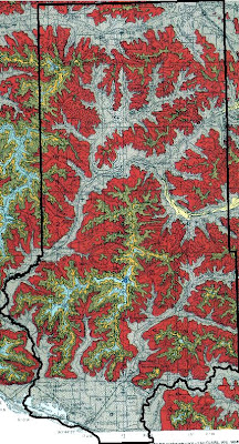Fig. 2 - Geologic formations which can help indicate best areas for mining silica sand.

Since this data could not be found in digital format, we had to use a scanned map. For this reason, we cannot determine their locations using just the map. The way around this is to determine if there is a relationship between elevation and the geologic formations using a DEM. Contour lines with 10m intervals were then propogated from the DEM to give us a digital feature to work with for identifying exact locations. Once this was done and we figured out the elevation ranges, we turned back to the DEM to reclassify it based on elevation rankings. It was apparent that the Jordon deposits were located at a higher elevation then the Wonewoc deposits therefore necessitating the higher elevations (340-416) to receive a rank of 3, intermediate elevations (260-340) a 2, and lowest elevations (194-260) a 1.

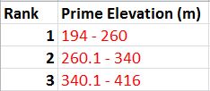Fig. 3 - Elevation class break table.

The Wonewock deposits were found in a combination of the three but mostly in the intermediate elevations. The classification method used was the Jenks Natural Breaks method since the elevations were pretty well distributed. The Reclassify tool was added to Model Builder and the parameters set to those mentioned above.

Fig. 4 - Model used to reclassify the elevation ranges.

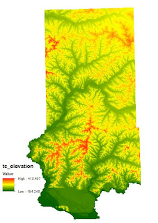Fig. 5 - Elevation range of Trempeleau County.

The task for Objective 2 was to find suitable land based on land use criteria. A land use/land cover (LULC) map for Trempeleau County was downloaded from the National Land Cover Dataset (NLCD). The image was classified into: Water, Urban/Built-Up, Barren, Agriculture, Herbaceous/Shrub, Forest, and Wetlands. The determining factor in ranking the LULC was the effort required to clear the land for a sand mine. Since Water, Urban/Built-Up, and Wetlands are obviously inappropriate locations for a mine location, they received a rank of 0. Forest was considered the most difficult to prepare and clear for a sand mining so it received a rank of 1. Herbaceous/Shrubland is listed as grasslands or shrubs with a canopy less than 5m tall. This type of land would be relatively easy to clear so it received a rank of 2. Finally, Barren and Agriculture are already cleared lands to these would be the best locations and they were given a rank of 3.

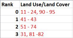Fig. 6 - LULC class break table via codes from LULC Classification Legend below.

An argument could be made that agricultural land should be preserved based on it's productivity purposes but it was felt that since we are looking at the effort needed to clear the land it would be given the highest rank.

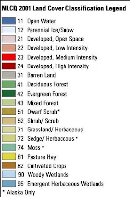Fig. 6 - NLCD 2001 LULC legend used to determine  areas of suitability.

Fig. 6 - Model used to reclassify the LULC raster into a suitability rank.

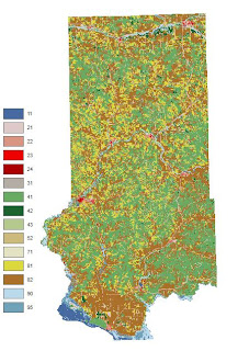Fig. 7 - Land Use/Land Cover (LULC) of Trempeleau County.

Objective 3 wanted us to find suitable land for the proximity to railroads. Finding distance to railroads is not practical since you can't load the rail cars at any given point on the rail. Therefore, instead of using railroads, rail terminals was used instead because these are the loading stations. For this process, the Euclidean distance needed to be used. Euclidean distance gives an output of straightline distance from a vector feature class. There are no rail terminals located within Trempeleau County. There is a terminal to the north and a terminal to the south of which are the closest to any location within Trempeleau County. Since Euclidean Distance is only run to the extent of the furthest feature, a portion of Trempeleau County was left out.

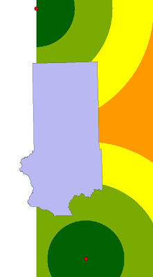Fig. 8 - Euclidean Distance from rail terminals which left out a portion of Trempeleau County.

A query was run to extract the counties surrounding Trempeleau County so that the Euclidean distance would cover the whole county based on the target rail terminals.

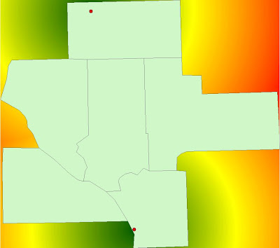Fig. 9 - Euclidean Distance was run again to ensure full coverage of Trempeleau County.

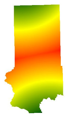Fig. 10 - The raster above was the masked to the extent of Trempeleau County.

The next step was to reclassify the Euclidean Distance based on the distance from rail terminals. Once again the Natural Breaks method was used to determine class breaks for the distances. The shortest distance range (13-21 miles) was ranked highest at 3. The intermediate distance (21.1-29 miles) was given a rank of 2 and the furthest distance (29.1-37 miles) was given a ranking of 1.

Fig. 11 - Class break table based on Euclidean Distance.

Fig. 12 - Model showing the workflow of masking and reclassifying the raster based on Euclidean Distance.

For Objective 4, we needed to find suitable land based on slope. The DEM stores elevation data and can be utilized give an output with calculated slope. The output value was set to "percent rise" to ensure this. The output was very detailed and contained a "salt and pepper" look. The slope values needed to be averaged out to give the raster a smoother look. The appropriate tool to do this is called Focal Statistics. This tool passes a 3x3 cell window over the raster to average out the values.

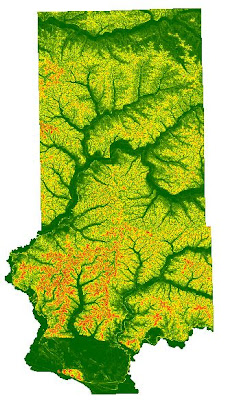Fig. 13 - The original slope output containing the "salt and pepper" look.

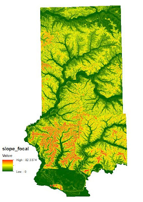Fig. 14 - Slope raster after being filtered to average out slope values giving it a smoother appearance.

After the Focal filter had been passed over the raster, the next step was to reclassify the raster based on slope values. It was determined that the more desirable locations would be located in areas with a lower slope gradient. Therefore the class breaks were as follows: low slope (0-10) was ranked at 3, medium slope (10.1-25) a rank of 2, and high slope (25.1-82) a rank of 1.


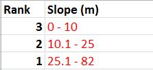Fig. 15 - Slope criteria table rank.

Fig. 16 - Workflow to average slope values and then to reclassify it for suitability.

The 5th and final objective was to assess suitability based on water table depth. Mining companies prefer to build their mines on a location where the water table is close to the surface. A water table elevation map was downloaded from the Wisconsin Geological Survey in the form of a coverage (e00). This type of file is not directly supported in ArcMap. It was necessary to import this coverage running a tool called "Import from e00 (Conversion)". This tool will convert the coverage into an arc feature class so that it will then be compatible with the ArcMap software. Since this is a contour feature class, it is a vector, so it was necessary to convert the contours into a raster so that it could be used for analysis with the other rasters. The tool used for this conversion is called "Topo to Raster" which interpolates a hydrologically correct raster surface from point, line, and polygon data. The value field was set to the Water Table Depth field and type set to Contours.

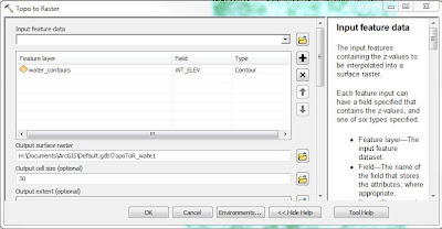Fig. 17 - The Topo to Raster tool was used to convert a contour feature into a raster.

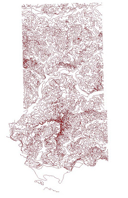Fig. 18 - Imported contour line file for water depth table.

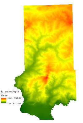Fig. 19 - Top to Raster conversion.

Fig. 20 - Water table depth reclassification model.

The classification method used on the water depth table was to break the range of values into three classes using Natural Breaks. The classes were then ranked as follows: (611-780) was given a 3, (780.1-930) a 2, and (930.1-1125) a 1.

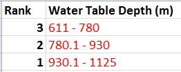Fig. 21 - Table ranking water table depth criteria.

Results/Discussion

Below are the ranked rasters for each objective stated above. Remember that a 3 means best location and a 1 means poor location. A value of 0 means that these areas are off limits.

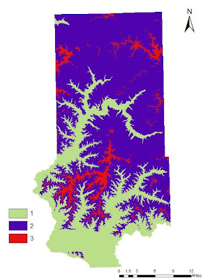Fig. 22 - Elevation ranked according to geologic deposit locations.

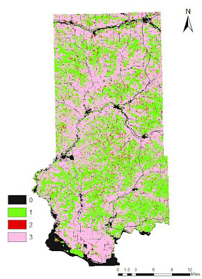Fig. 23 - Reclassified LULC raster showing the ranked areas of suitability.

The areas containing a 0 value are regions defined as water, wetlands, and urban. These areas are off limits.

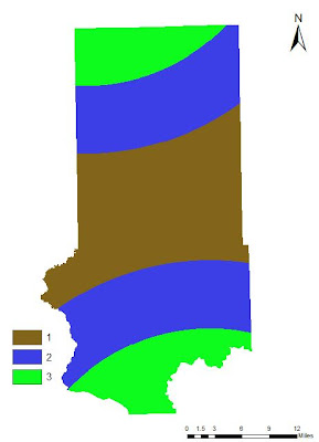Fig. 24 - Reclassified raster showing ranked Euclidean Distance from rail terminals.

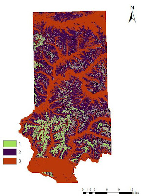Fig. 25 - Ranked suitability raster for slope.

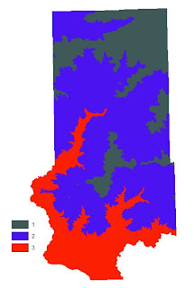Fig. 26 - Water table depth rank.

The 5 ranked suitability rasters were then added together via the Raster Calculator tool. This tool adds together the ranked values of each pixel on each raster and then creates a new raster containing the summed up values. The lowest possible value is a 5 and the highest value can be a 15 (3x5).

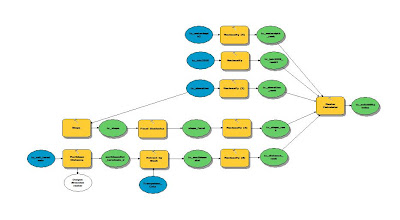Fig. 27 - Raster Calculator used to sum up all of the criteria rasters.

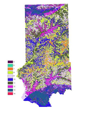Fig. 28 - Ranked Suitability Index based on 5 criteria.

It turns out that there is no location in which the maximum suitability exists on all 5 rasters so the highest ranking is a 14 vs. a 15. It was then necessary to make the LULC raster into binary so areas of residential, water, and wetlands are given a 0 value and all other acceptable areas a 1. This was then multiplied by the raster in Fig. 25 so that areas off limits for a sand mine are then coded as 0 and all other values retain their original values. The Index was then reclassified into 3 classes: (5-7) = 1, (8-10) = 2, and (11-14) = 3.


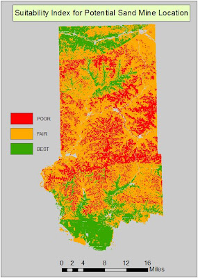Fig. 29 - Final Suitability Index map.

Since the class breaks were defined using the discretion of the modeler, the output can vary depending on how the user breaks the classes up for suitability. For this reason, the results can be very subjective. This is why the user needs to have a reason for how the classes are broken up as it can alter the output. That being said, I am very confident with my decisions in that regard and believe the output Suitability Index illustrates a logical data flow and can be implemented in a plan for finding optimal locations for a new sand mine.

Conclusion

This exercise was a very valuable learning experience as we got a chance to use skills learned in the classroom and apply them to a real world situation. This project was a lot of fun to work on especially being given the responsibilities of downloading the data, setting up environments, using logic, and building models to expedite the processes involved. A few speed bumps were encountered along the way but figuring out what is causing the problem and being able to fix it allows the user to develop great troubleshooting skills.